The Fundamental Theorem of Calculus
Today we are walking through a subject that many people have fear of. I’m talking about calculus. Although hearing about derivatives and integrals may be a bit shocking at first, the reality is that it is simply amazing when you understand it. If you are not familiar with calculus or math, don’t worry, we will explain it all in a conceptual way.
Let’s start thinking about a circle. We learned that the area of a circle is calculated using the formula 2 * PI * r , where r is the radius of the circle. But where does this come from? Let’s divide our circle in many rings, like this:

For this purpose, we will call the thickness of the ring dr . We can think of a ring as a coiled line. If we uncoil it, we will see that the figure is similar to a rectangle, so we approximate this ring to a rectangle. That said, our thickness would be the rectangle height, and 2 * PI * r (the formula to the cirfumfere) is the rectangle width. So the area of our rectangle approximation is 2 * PI * r * dr. But as dr becomes smaller (which means as we slice our circle in smaller and smaller rings), the approximation will become less and less wrong.
Note that we divided our circle in many rings, so it’s logical to conclude that the area of our circle is the sum of the area of all rings. A way to visualize this is to plot a graph from 0 to r, with columns that represent our rings.
If we choose smaller and smaller values for dr, the area of our rectangles keeps getting closer of the precise area under the graph. The portion under the graph is a triangle, whose base is 1, and height is 2 * PI * 1 . So the area, which is (base * height) / 2 comes out to be PI *1² . Or, if the radius of our original circle had been other value R, area = 1/2 * R * 2 * PI * R = PI * R²
Integrals
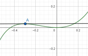
Imagine we have the following graph for the function f(t) = t³:
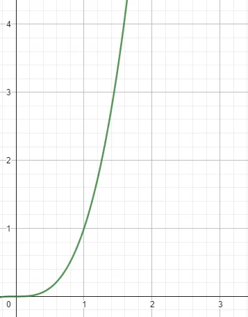
Now, we set the left endpoint at the origin (0), but let’s think that the right endpoint (that we will call x) varies. How can we describe the area under the graph of f(t) when we consider the variation of our endpoint x?
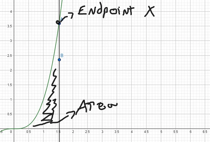
We do it the following way:

In mathematics, integral is a concept used to calculate the area under a curve or the total accumulated value of a function over an interval. Consider a linear function such as f(x) = 2. This function is represented graphically like this:
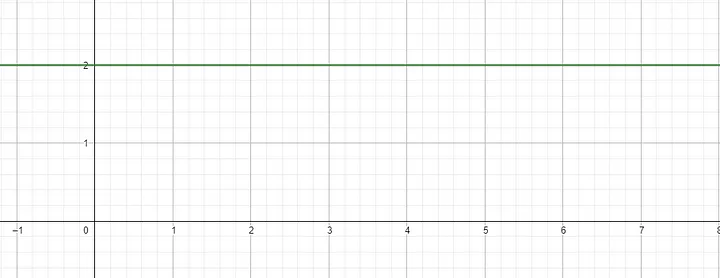
To calculate the area under our function, we simply calculate the area of the rectangle formed by the height of the function over that interval and the width of the interval itself.
However, we may deal with more complex functions, like polynomials. Imagine a function like the one below:
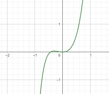
In that case, it is impossible to calculate the area using simple geometry, like we did before. Instead, we use integration to approximate the area under the curve. Integration involves dividing the area under the curve into an infinite number of small rectangels, with an infinitelly small width and then summing up the area of all rectangles. The result is approximately the total area under the curve, like we represented using our circle rings. This is the foundation of the theory of integration.
Derivatives
Derivatives are usually defined as “instantaneous rate of change”, but think about this definition for a second. Things only change if we measure different points in time. Think about a moving car: what if I told you that our car is moving 60km per hour, and asked what is the velocity of our car at the instant i?
You cannot measure how fast the car was at a single instant, because there is no room for change since we don’t have separate points in time. Velocity itself is the distance traveld over a given amount of time, so this is a paradox. But we have speedometers right? When you are driving, the car shows your speed at a given moment… or this is what it appears to happen. In reality, the car system is computing speed during very small amounts of time.
This means that if we choose a small amount of time dt, we can compute the rise over the run:

The idea presented here is almost what a derivative is. Although a car will choose a small amount like 0.001 seconds to compute speed, in math, the derivative is not this ratio for a specific choice of dt. It’s whatever value this ratio approaches as the choice for dt approaches 0.
Another way to think about ds/dt is the slope of the line passing through two points on the graph. The derivative is equal to the slope of a line tangent to the graph at a single point.
For example, let’s think about a linear function, such as f(x) = 2x + 2 . Knowing the concept of derivatives, we can compute the derivative of our function easily. The graph for this function looks like this:
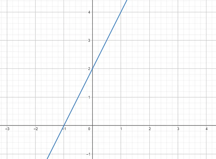
It doesn’t matter the value of x, the slope of the line will always be 2 (because in linear equations of form f(x) = ax + b, a represents the linear coefficient that dictates the slope of the line. In our case, it its one). Derivatives of constant values, such as our b are 0, because there is no change in constant values. That said, the derivative of a linear function is it’s linear coefficient a. In our case, note that every time we increase X by 1 unit, the value of the function increases by 2 units, so the rate of change is always the same.
There are a lot of techniques to computing derivatives for other types of functions, such as power, exponential, logarithmic and so on. I will not cover those in this article since it is mostly conceptual.
The formal definition of a derivative is that the derivative of y with respect to x is defined as the change in y over the change in x as the distance between x0 and x1 becomes smaller and smaller. [source]

This is the math definition of a derivative, which is the slope of the tangent line to the graph of f(x) in that point, it measures how quickly the value of f(x) changes with small changes in x.
Fundamental Theorem of Calculus
After all we’ve been through in this article, this is the time to stitch it all together and understand the relation between the slope of a curve and the area below it, the Fundamental Theorem of Calculus. It states that integration (integrals) and differentiation (derivatives) are inverse operations of each other.
It states that for a function f , an antiderivative may be obtained as the integral of f over an interval with a variable upper bound.
Quick definition: antiderivatives (also known as indefinite integrals) of a function f is a differentiable function F whose derivative is equal to the original function f. (F’ = f).
Basically, if function f(x) is continuous over an interval I, and if F(x) is any antiderivative of f(x) over that interval I, then the indefinite integral of f(x) is F(x) + integration constant. In other words, integration undoes differentiation and restores the original function up to an arbitrary constant. This is what states that they are inverse operations of each other.
The theorem also states that the integral of f over a fixed interval is equal to the change of any antiderivative F between the ends of the interval. It simplifies the calculation of a definite integral.
Simply amazing.
Thanks for reading, see you next week!
Lorenzo
References
Howard A, Irl C. B Bivens, Sephen L. Davis; et al. Cálculo.v1, 10th ed. Bookman, 2014.